- 文章信息
- 作者: kaiwu
- 点击数:777
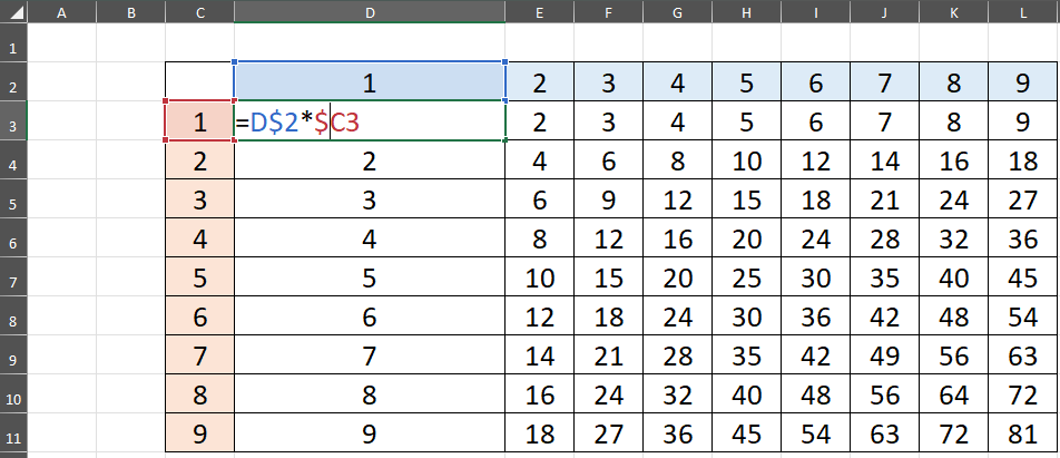
1.九九表

工作簿:http://kaiwu.city/openfiles/excel_reference.xlsx
工作表:30cities
任务:做得快的同学,研究一下如何计算30城市二者之间的距离
=SQRT(POWER(M$2-$I6,2)+POWER(M$3-$J6,2))
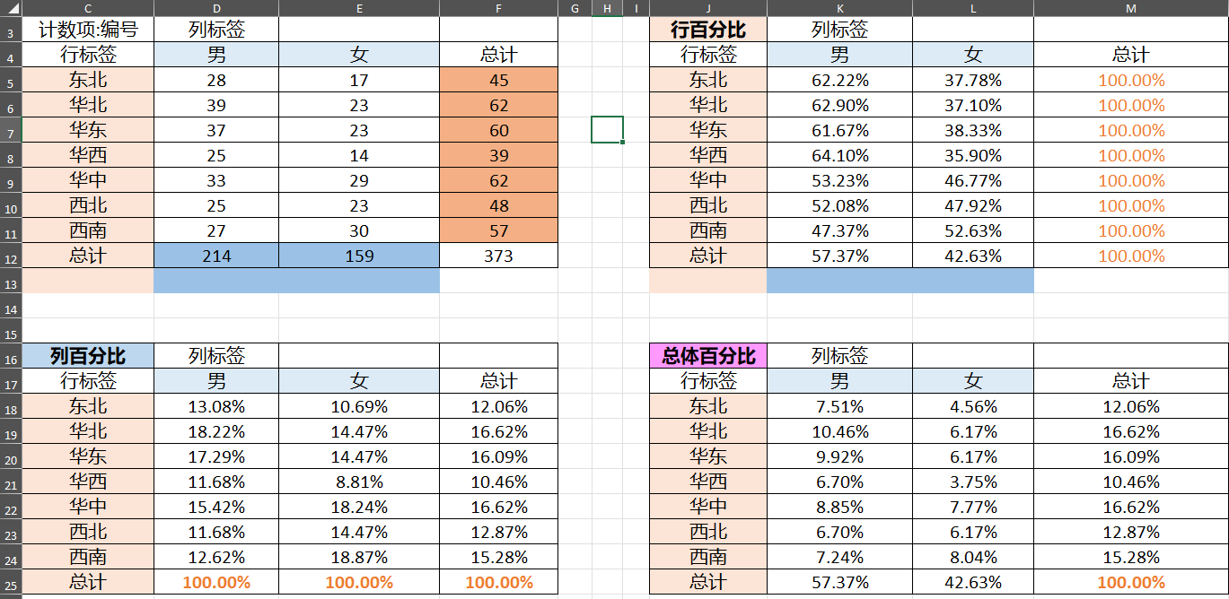
2.三种百分比
工作簿:http://kaiwu.city/openfiles/excel_reference.xlsx
工作表:crosstable
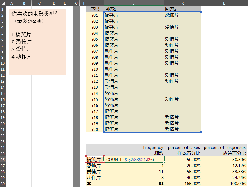
3.多选题
工作簿:http://kaiwu.city/openfiles/excel_reference.xlsx
工作表:multi_response
4.数据透视表
分类变量包含标签的Excel文件 (有 variable labels变量名标签和 value labels变量值标签)
http://kaiwu.city/openfiles/data_tourist_with_cnlabels.xlsx
(1)频数分析
性别、
5.VBA
http://kaiwu.city/openfiles/Excel_VBA_example.xlsm
http://kaiwu.city/index.php/vba
- 文章信息
- 作者: kaiwu
- 点击数:125
1. basic of excel
http://kaiwu.city/index.php/online-office-en
![]()
![]()
tengxun document
![]()
2.download the simulated dataset

2.1 questionnaire(simulated dataset)
2.2 data for general purpose (without variable labels and value labels)

2.3 data for Excel (with variable labels and value labels)
http://kaiwu.city/openfiles/data_tourist_satisfaction_enlabels2024.xlsx
- 文章信息
- 作者: kaiwu
- 点击数:285


- 文章信息
- 作者: kaiwu
- 点击数:568
可以通过anaconda安装python(http://kaiwu.city/index.php/python),操作极为简单;但是anaconda程序很大,而且其包含的python及python拓展模块library不是最新的版本。
![]()
![]()
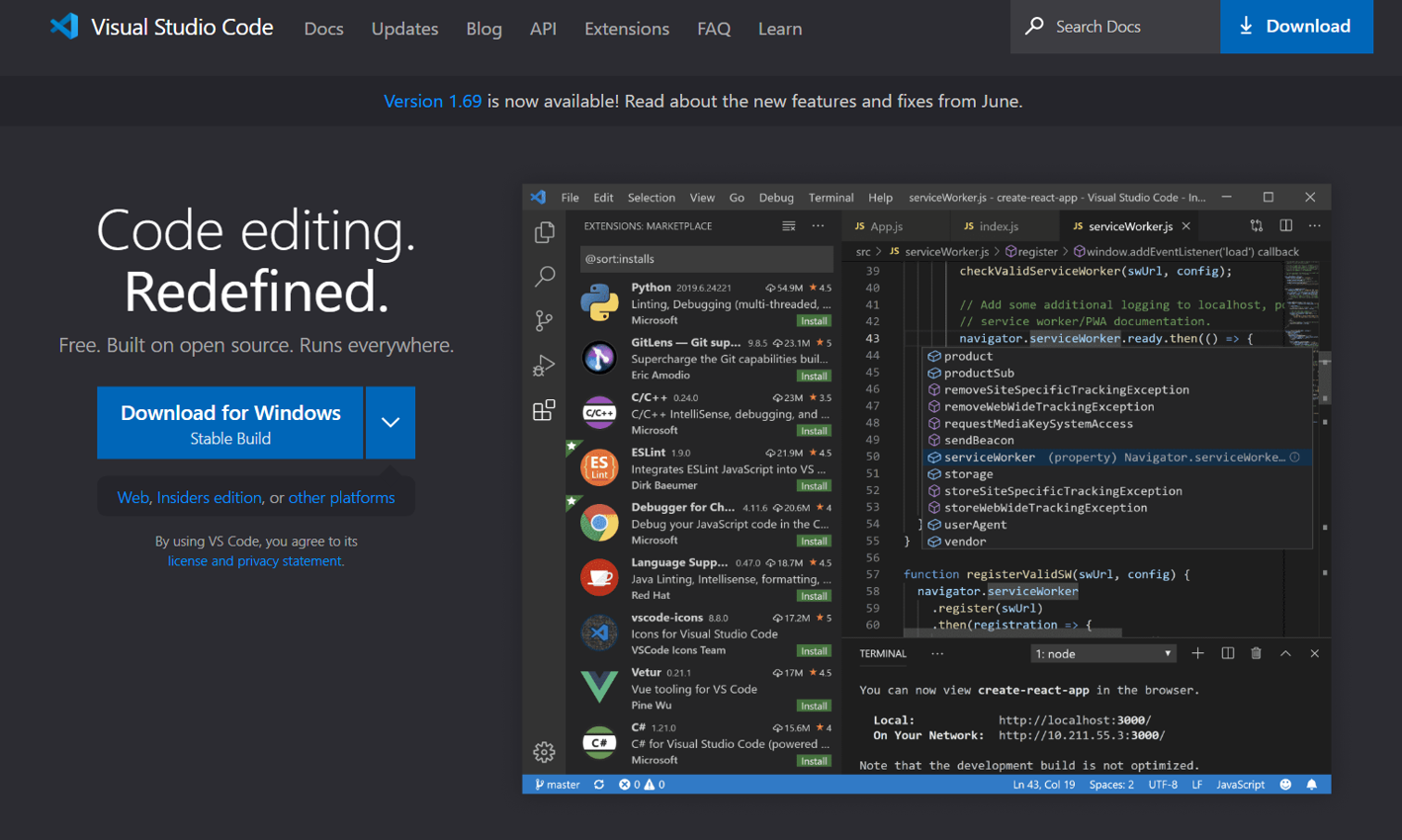
直接安装python,并以微软的开源软件 Visual Studio Code(https://code.visualstudio.com/)作为IDE是不错的选择。
![]()
微软提供了详细的安装指南
https://docs.microsoft.com/en-us/learn/modules/python-install-vscode/
Get started with Python in Visual Studio
Get started with learning Python by installing and configuring the tools you'll need to build real applications.
Learning objectives
By the end of this module, you'll be able to:
- Install Python 3, if needed.
- Install and configure Visual Studio Code and extensions on your computer.
- Create a Python file.
- Write and run Python code in Visual Studio Code.
Prerequisites
- Ability to install programs locally.
- Basic familiarity with programming concepts.
This module is part of these learning paths
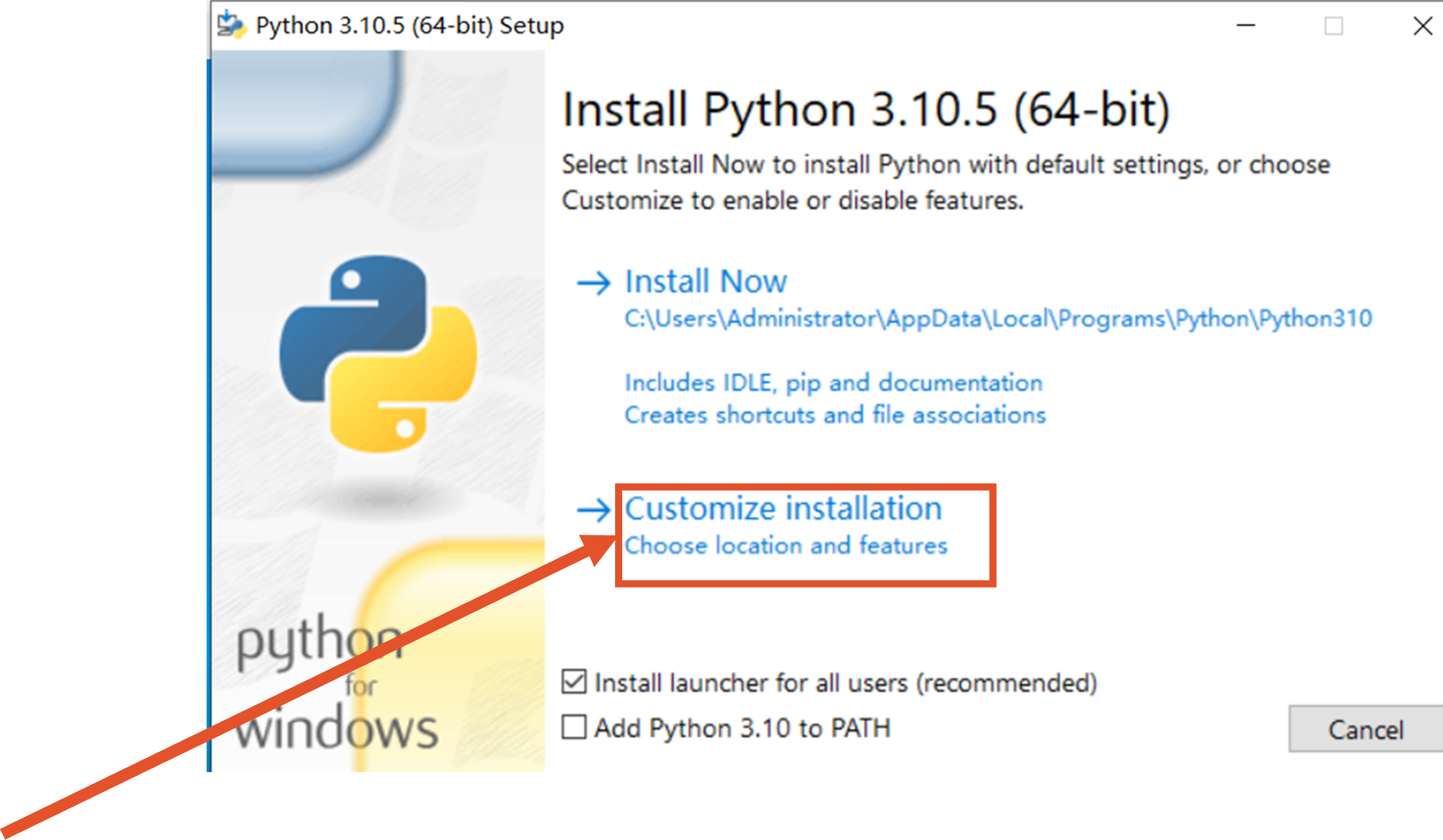
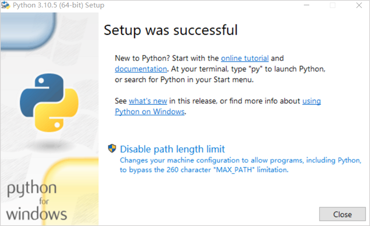
1.安装python
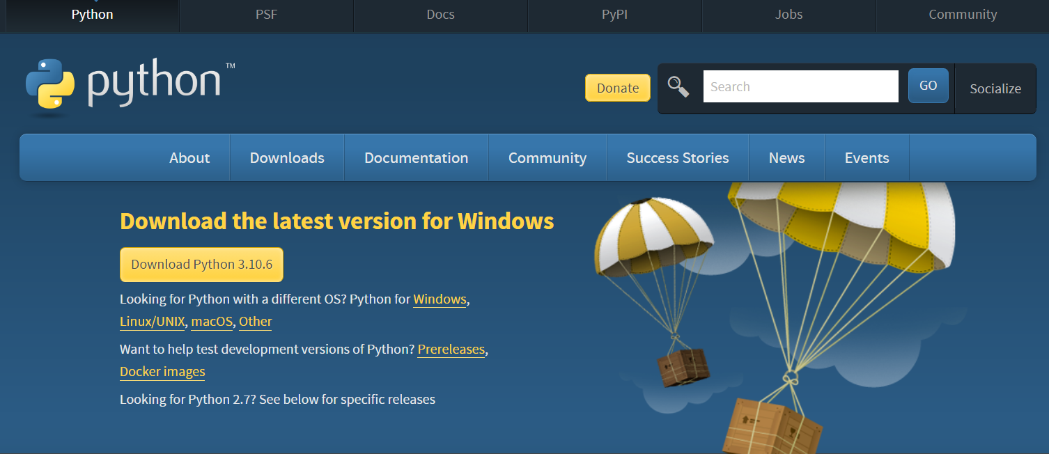
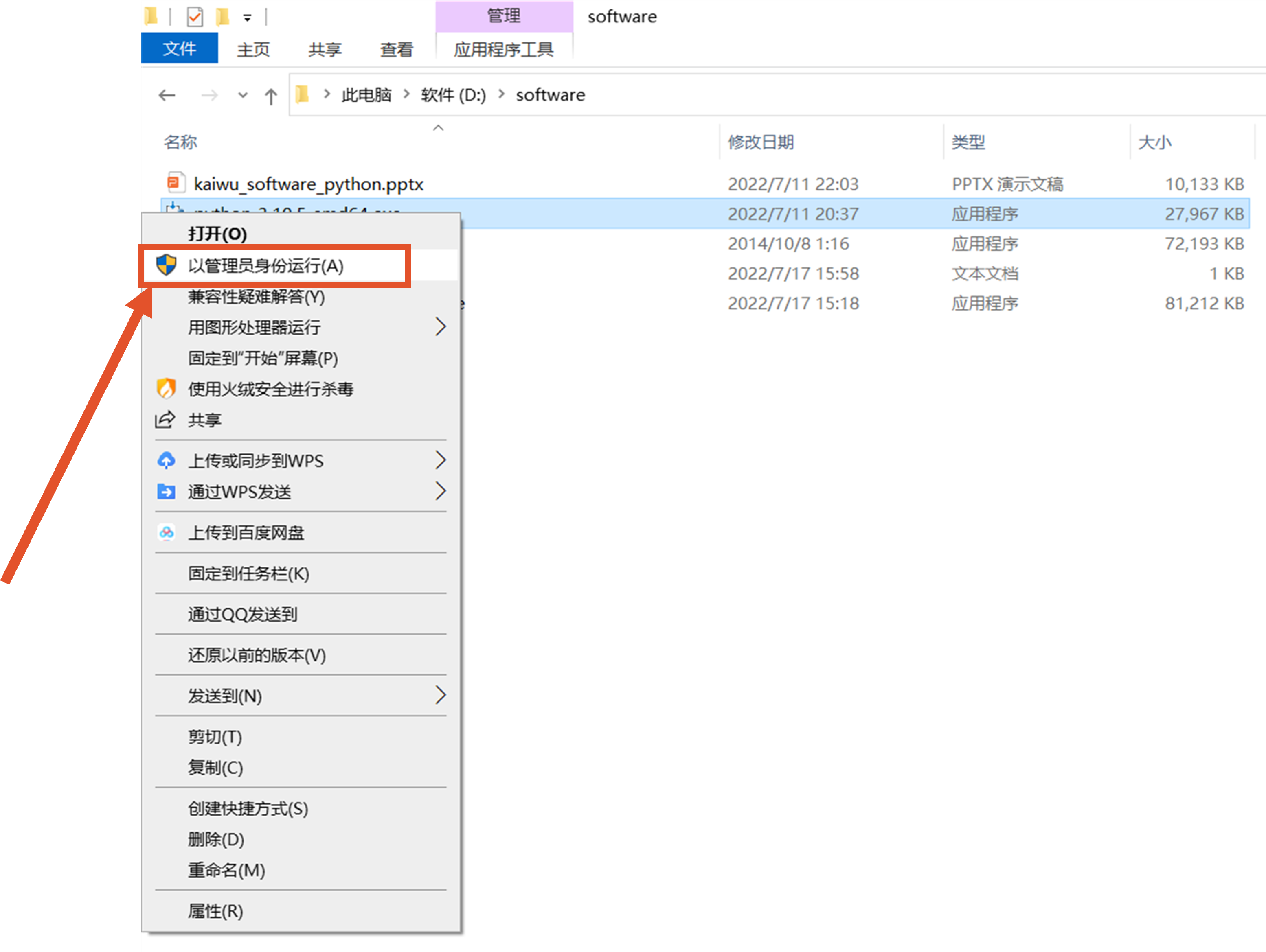
访问python官网,下载安装程序
https://www.python.org/downloads/


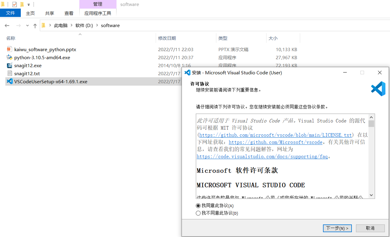
2.安装VScode
https://code.visualstudio.com/
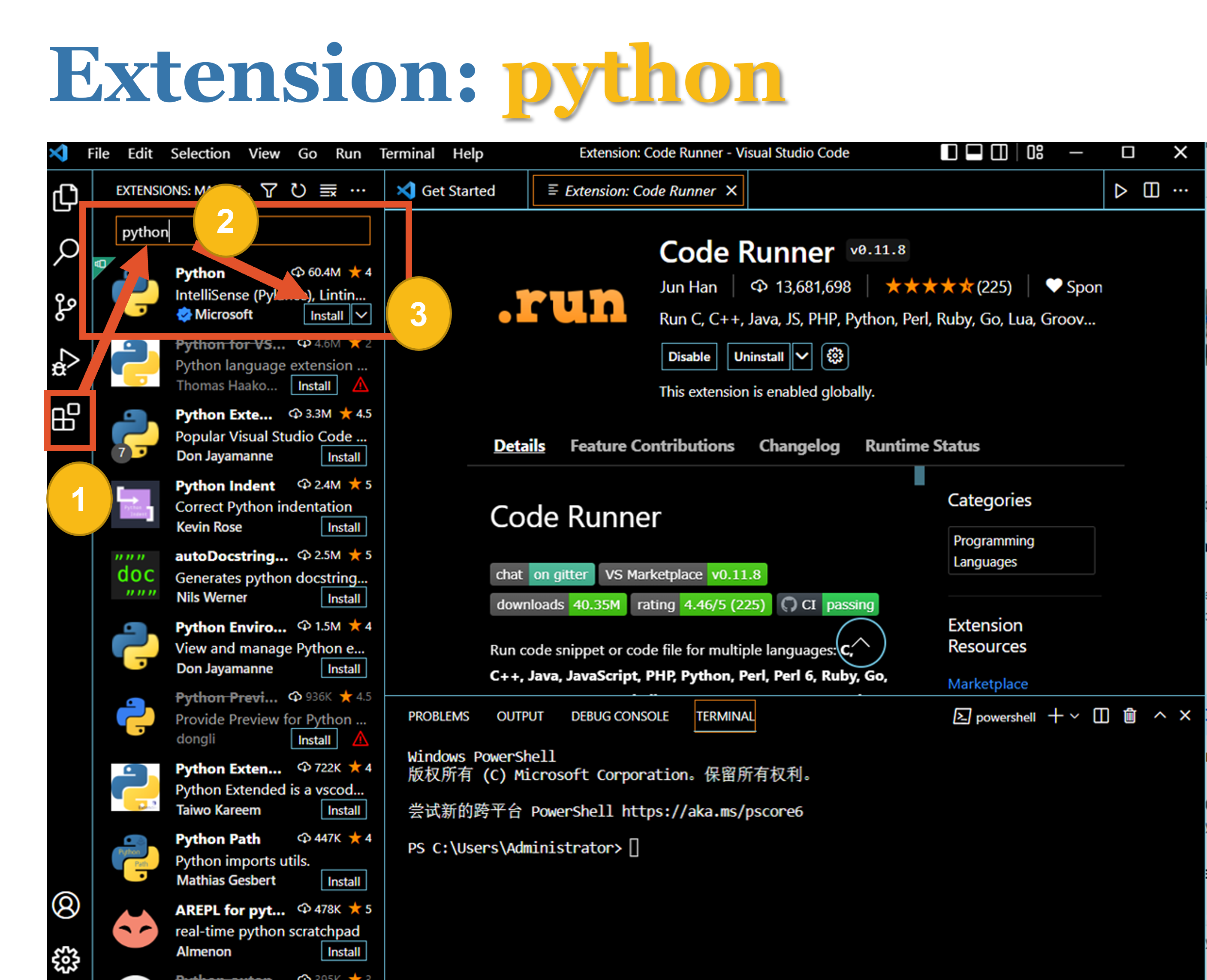
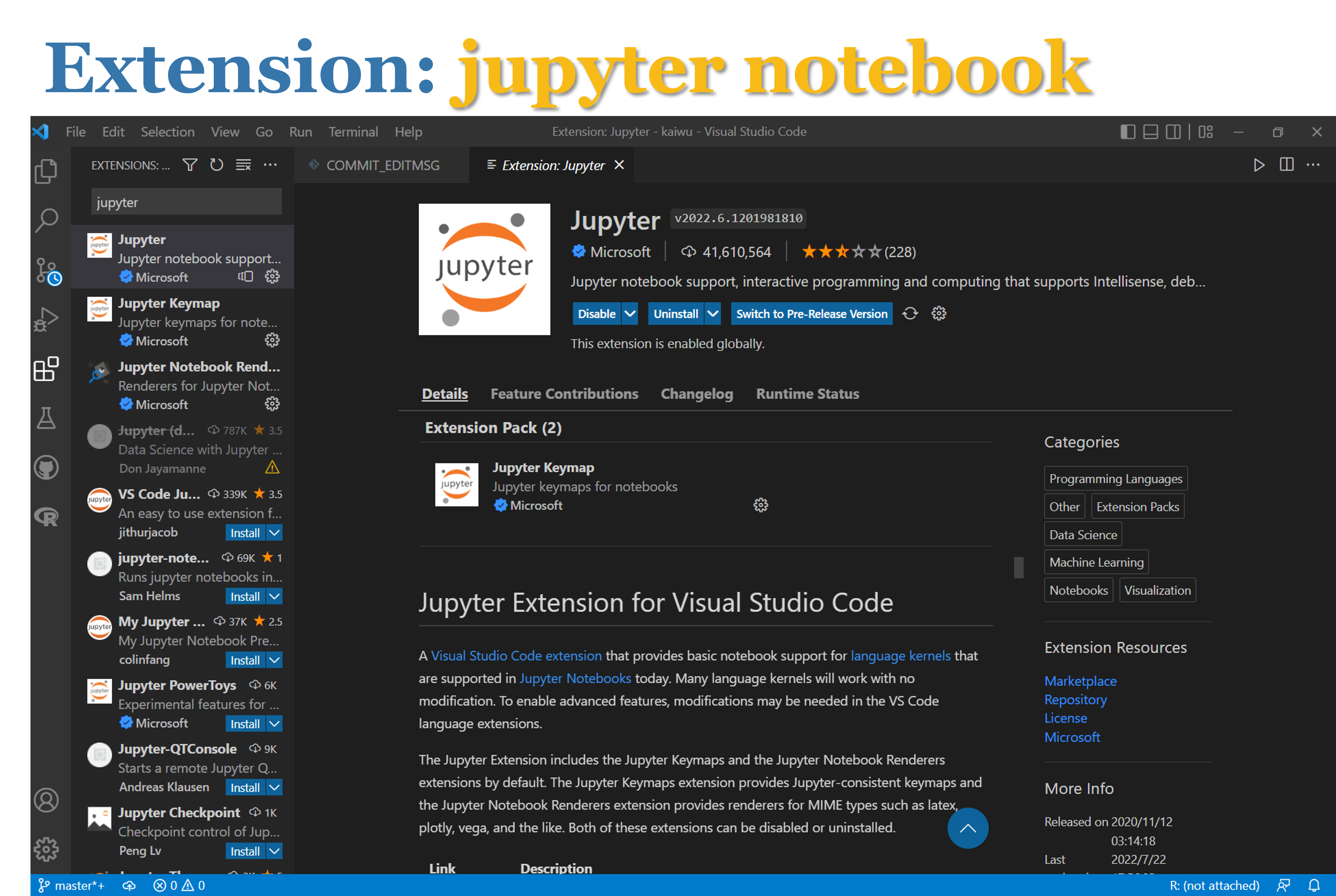
3.安装VScode的拓展程序
(1)code runner
(2)python
(3)jupyter notebook

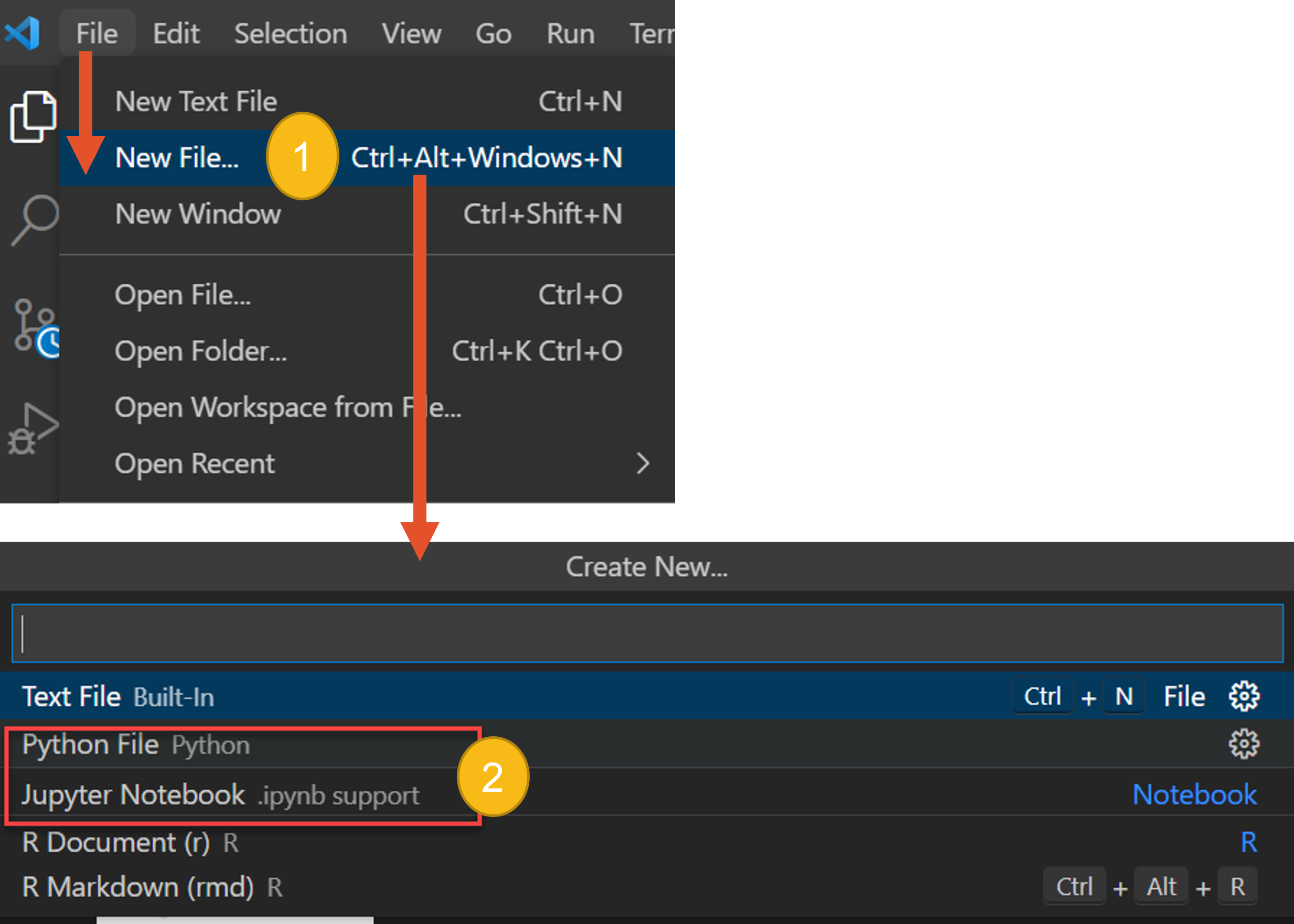
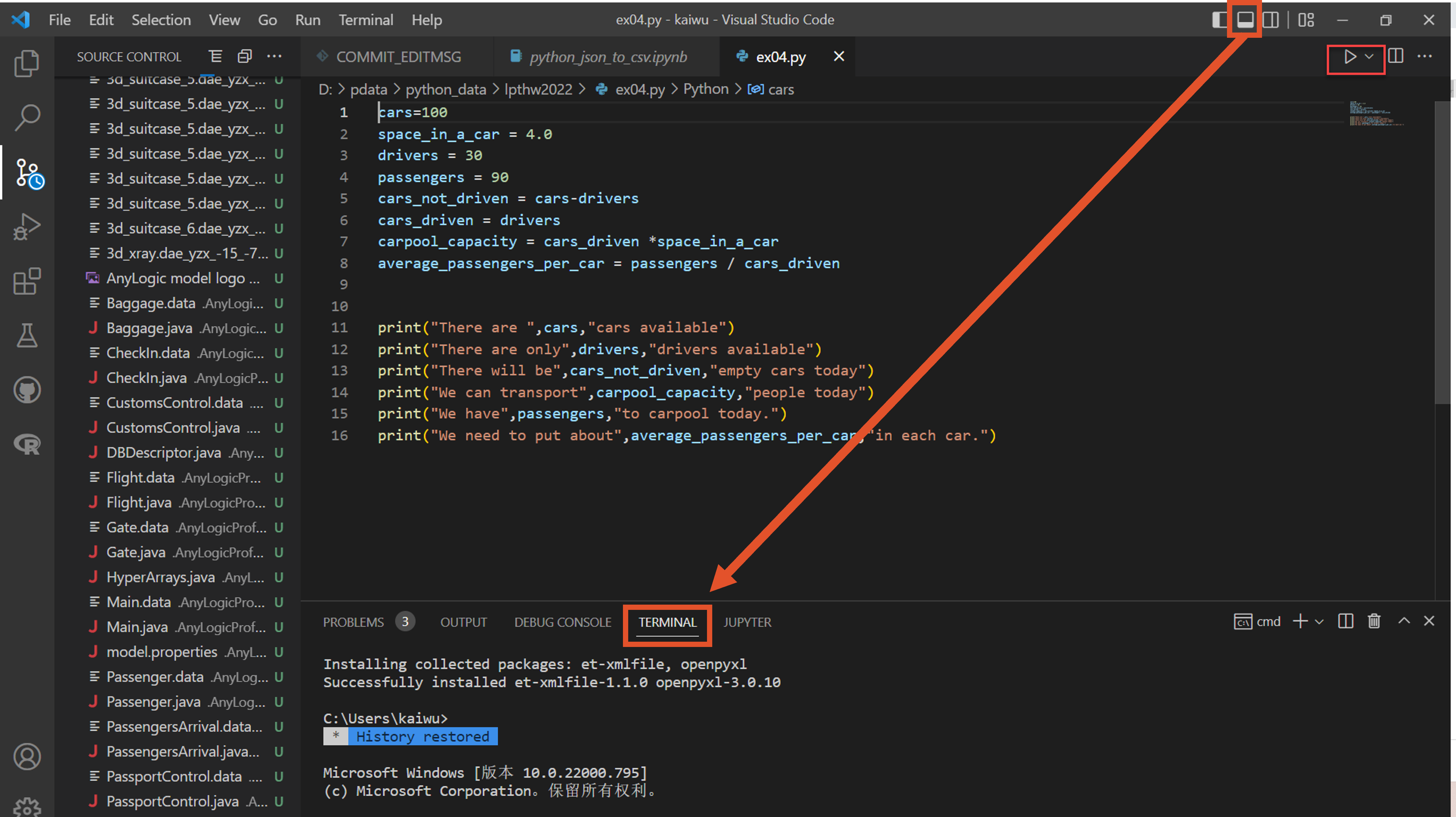
4.以vscode作为IDE,新建、编辑、运行python程序
- 文章信息
- 作者: kaiwu
- 点击数:580
1.ollama
https://github.com/ollama/ollama
https://ollama.com/blog/llama3

用于ollama的模型:
Ollama supports a list of models available on ollama.com/library
Here are some example models that can be downloaded:
| Model | Parameters | Size | Download |
|---|---|---|---|
| Llama 3.2 | 3B | 2.0GB | ollama run llama3.2 |
| Llama 3.2 | 1B | 1.3GB | ollama run llama3.2:1b |
| Llama 3.1 | 8B | 4.7GB | ollama run llama3.1 |
| Llama 3.1 | 70B | 40GB | ollama run llama3.1:70b |
| Llama 3.1 | 405B | 231GB | ollama run llama3.1:405b |
| Phi 3 Mini | 3.8B | 2.3GB | ollama run phi3 |
| Phi 3 Medium | 14B | 7.9GB | ollama run phi3:medium |
| Gemma 2 | 2B | 1.6GB | ollama run gemma2:2b |
| Gemma 2 | 9B | 5.5GB | ollama run gemma2 |
| Gemma 2 | 27B | 16GB | ollama run gemma2:27b |
| Mistral | 7B | 4.1GB | ollama run mistral |
| Moondream 2 | 1.4B | 829MB | ollama run moondream |
| Neural Chat | 7B | 4.1GB | ollama run neural-chat |
| Starling | 7B | 4.1GB | ollama run starling-lm |
| Code Llama | 7B | 3.8GB | ollama run codellama |
| Llama 2 Uncensored | 7B | 3.8GB | ollama run llama2-uncensored |
| LLaVA | 7B | 4.5GB | ollama run llava |
| Solar | 10.7B | 6.1GB | ollama run solar |
Note
You should have at least 8 GB of RAM available to run the 7B models, 16 GB to run the 13B models, and 32 GB to run the 33B models.
2.中文相关的几个模型
2.1 llama2-chinese
https://ollama.com/library/llama2-chinese
ollama run llama2-chinese
2.2 qwen
https://ollama.com/library/qwen
阿里云的千问模型
ollama run qwen
2.3 yi
Yi 是百度的大语言模型
https://ollama.com/library/yi:34b
https://huggingface.co/01-ai/Yi-34B
ollama run yi
ollama run yi:9b
ollama run yi:34b
3.图形界面
https://github.com/fmaclen/hollama
一个用于与 Ollama 服务器对话的简约网页界面。
功能特点:
- 大型提示字段
- 支持语法高亮的 Markdown 渲染
- 代码编辑器功能
- 可定制的系统提示
- 复制代码片段、消息或整个会话
- 编辑并重试消息
- 数据本地存储在您的浏览器上
- 响应式布局
- 浅色和深色主题
- 多语言界面
- 直接从界面下载 Ollama 模型
 |
|---|
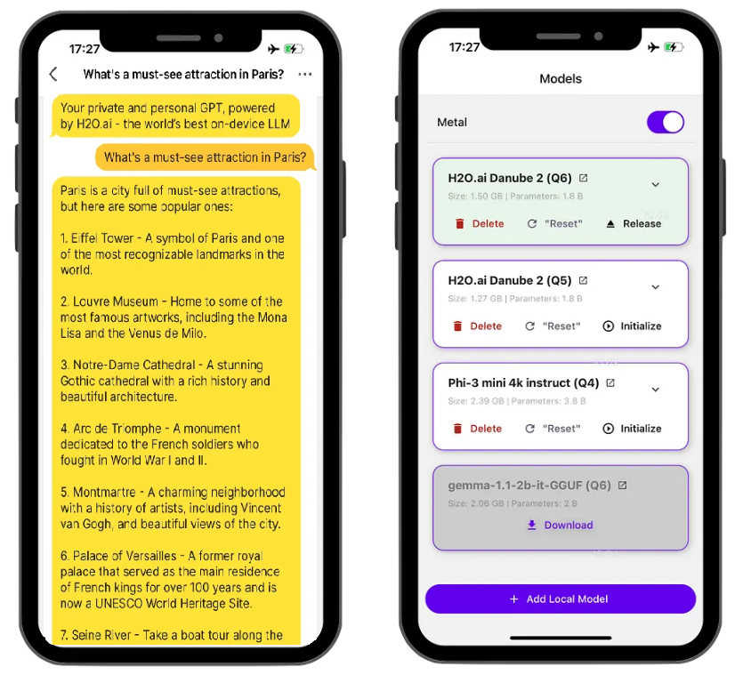
4.移动应用app
Pocketpal这个app可以下载LLama模型,可以在没有联网的情况下(手机本地环境)进行类似于chat GPT的问答
https://github.com/Anicodeth/Pocketpal/tree/main/Mobile
https://github.com/a-ghorbani/PocketPal-feedback
https://apkpure.com/cn/pocketpal/com.pocketpalai/
PocketPal_1.4.6_APKPure.xapk
![]()
https://play.google.com/store/apps/details?id=com.pocketpalai